Data Structures & Algorithms - Quick Guide (Step By Step) (1)

 Overview

Data Structure is a systematic way to organize data in order to use it efficiently. Following terms are the foundation terms of a data structure.

• Interface − Each data structure has an interface. Interface represents the set of operations that a data structure supports. An interface only provides the list of supported operations, type of parameters they can accept and return type of these operations.

• Implementation − Implementation provides the internal representation of a data structure. Implementation also provides the definition of the algorithms used in the operations of the data structure.

Characteristics of a Data Structure

• Correctness − Data structure implementation should implement its interface correctly.

• Time Complexity − Running time or the execution time of operations of data structure must be as small as possible.

• Space Complexity − Memory usage of a data structure operation should be as little as possible.

Need for Data Structure

As applications are getting complex and data rich, there are three common problems that applications face now-a-days.

• Data Search − Consider an inventory of 1 million(106) items of a store. If the application is to search an item, it has to search an item in 1 million(106) items every time slowing down the search. As data grows, search will become slower.

• Processor speed − Processor speed although being very high, falls limited if the data grows to billion records.

• Multiple requests − As thousands of users can search data simultaneously on a web server, even the fast server fails while searching the data.

To solve the above-mentioned problems, data structures come to rescue. Data can be organized in a data structure in such a way that all items may not be required to be searched, and the required data can be searched almost instantly.

Execution Time Cases

There are three cases which are usually used to compare various data structure's execution time in a relative manner.

• Worst Case − This is the scenario where a particular data structure operation takes maximum time it can take. If an operation's worst case time is ƒ(n) then this operation will not take more than ƒ(n) time where ƒ(n) represents function of n.

• Average Case − This is the scenario depicting the average execution time of an operation of a data structure. If an operation takes ƒ(n) time in execution, then m operations will take mƒ(n) time.

• Best Case − This is the scenario depicting the least possible execution time of an operation of a data structure. If an operation takes ƒ(n) time in execution, then the actual operation may take time as the random number which would be maximum as ƒ(n).

Basic Terminology

• Data − Data are values or set of values.

• Data Item − Data item refers to single unit of values.

• Group Items − Data items that are divided into sub items are called as Group Items.

• Elementary Items − Data items that cannot be divided are called as Elementary Items.

• Attribute and Entity − An entity is that which contains certain attributes or properties, which may be assigned values.

• Entity Set − Entities of similar attributes form an entity set.

• Field − Field is a single elementary unit of information representing an attribute of an entity.

• Record − Record is a collection of field values of a given entity.

• File − File is a collection of records of the entities in a given entity set.

Data Structures - Algorithms Basics

Algorithm is a step-by-step procedure, which defines a set of instructions to be executed in a certain order to get the desired output. Algorithms are generally created independent of underlying languages, i.e. an algorithm can be implemented in more than one programming language.

From the data structure point of view, following are some important categories of algorithms −

• Search − Algorithm to search an item in a data structure.

• Sort − Algorithm to sort items in a certain order.

• Insert − Algorithm to insert item in a data structure.

• Update − Algorithm to update an existing item in a data structure.

• Delete − Algorithm to delete an existing item from a data structure.

Characteristics of an Algorithm

Not all procedures can be called an algorithm. An algorithm should have the following characteristics −

• Unambiguous − Algorithm should be clear and unambiguous. Each of its steps (or phases), and their inputs/outputs should be clear and must lead to only one meaning.

• Input − An algorithm should have 0 or more well-defined inputs.

• Output − An algorithm should have 1 or more well-defined outputs, and should match the desired output.

• Finiteness − Algorithms must terminate after a finite number of steps.

• Feasibility − Should be feasible with the available resources.

• Independent − An algorithm should have step-by-step directions, which should be independent of any programming code.

How to Write an Algorithm?  

There are no well-defined standards for writing algorithms. Rather, it is problem and resource dependent. Algorithms are never written to support a particular programming code.

As we know that all programming languages share basic code constructs like loops (do, for, while), flow-control (if-else), etc. These common constructs can be used to write an algorithm.

We write algorithms in a step-by-step manner, but it is not always the case. Algorithm writing is a process and is executed after the problem domain is well-defined. That is, we should know the problem domain, for which we are designing a solution.

Example

Let's try to learn algorithm-writing by using an example.

Problem − Design an algorithm to add two numbers and display the result.

Step 1 − START
Step 2 − declare three integers a, b & c
Step 3 − define values of a & b
Step 4 − add values of a & b
Step 5 − store output of step 4 to c
Step 6 − print c
Step 7 − STOP

Algorithms tell the programmers how to code the program. Alternatively, the algorithm can be written as −

Step 1 − START ADD
Step 2 − get values of a & b
Step 3 − c ← a + b
Step 4 − display c
Step 5 − STOP

In design and analysis of algorithms, usually the second method is used to describe an algorithm. It makes it easy for the analyst to analyze the algorithm ignoring all unwanted definitions. He can observe what operations are being used and how the process is flowing.

Writing step numbers, is optional.

We design an algorithm to get a solution of a given problem. A problem can be solved in more than one ways.

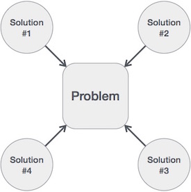
Hence, many solution algorithms can be derived for a given problem. The next step is to analyze those proposed solution algorithms and implement the best suitable solution.

Algorithm Analysis

Efficiency of an algorithm can be analyzed at two different stages, before implementation and after implementation. They are the following −

• A Priori Analysis − This is a theoretical analysis of an algorithm. Efficiency of an algorithm is measured by assuming that all other factors, for example, processor speed, are constant and have no effect on the implementation.

• A Posterior Analysis − This is an empirical analysis of an algorithm. The selected algorithm is implemented using programming language. This is then executed on target computer machine. In this analysis, actual statistics like running time and space required, are collected.

We shall learn about a priori algorithm analysis. Algorithm analysis deals with the execution or running time of various operations involved. The running time of an operation can be defined as the number of computer instructions executed per operation.

Algorithm Complexity

Suppose X is an algorithm and n is the size of input data, the time and space used by the algorithm X are the two main factors, which decide the efficiency of X.

• Time Factor − Time is measured by counting the number of key operations such as comparisons in the sorting algorithm.

• Space Factor − Space is measured by counting the maximum memory space required by the algorithm.

The complexity of an algorithm f(n) gives the running time and/or the storage space required by the algorithm in terms of n as the size of input data.

Space Complexity

Space complexity of an algorithm represents the amount of memory space required by the algorithm in its life cycle. The space required by an algorithm is equal to the sum of the following two components −

• A fixed part that is a space required to store certain data and variables, that are independent of the size of the problem. For example, simple variables and constants used, program size, etc.

• A variable part is a space required by variables, whose size depends on the size of the problem. For example, dynamic memory allocation, recursion stack space, etc.

Space complexity S(P) of any algorithm P is S(P) = C + SP(I), where C is the fixed part and S(I) is the variable part of the algorithm, which depends on instance characteristic I. Following is a simple example that tries to explain the concept −

Algorithm: SUM(A, B)
Step 1 -  START
Step 2 -  C ← A + B + 10
Step 3 -  Stop

Here we have three variables A, B, and C and one constant. Hence S(P) = 1 + 3. Now, space depends on data types of given variables and constant types and it will be multiplied accordingly.

Time Complexity

Time complexity of an algorithm represents the amount of time required by the algorithm to run to completion. Time requirements can be defined as a numerical function T(n), where T(n) can be measured as the number of steps, provided each step consumes constant time.

For example, addition of two n-bit integers takes n steps. Consequently, the total computational time is T(n) = c ∗ n, where c is the time taken for the addition of two bits. Here, we observe that T(n) grows linearly as the input size increases.

Data Structures - Asymptotic Analysis

Asymptotic analysis of an algorithm refers to defining the mathematical boundation/framing of its run-time performance. Using asymptotic analysis, we can very well conclude the best case, average case, and worst case scenario of an algorithm.

Asymptotic analysis is input bound i.e., if there's no input to the algorithm, it is concluded to work in a constant time. Other than the "input" all other factors are considered constant.

Asymptotic analysis refers to computing the running time of any operation in mathematical units of computation. For example, the running time of one operation is computed as f(n) and may be for another operation it is computed as g(n2). This means the first operation running time will increase linearly with the increase in n and the running time of the second operation will increase exponentially when n increases. Similarly, the running time of both operations will be nearly the same if n is significantly small.

Usually, the time required by an algorithm falls under three types −

• Best Case − Minimum time required for program execution.

• Average Case − Average time required for program execution.

• Worst Case − Maximum time required for program execution.

Asymptotic Notations

Following are the commonly used asymptotic notations to calculate the running time complexity of an algorithm.

• Ο Notation
• Ω Notation
• θ Notation

Big Oh Notation, Ο

The notation Ο(n) is the formal way to express the upper bound of an algorithm's running time. It measures the worst case time complexity or the longest amount of time an algorithm can possibly take to complete.

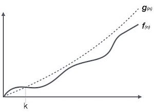
For example, for a function f(n)

Ο(f(n)) = { g(n) : there exists c > 0 and n0 such that f(n) ≤ c.g(n) for all n > n0. }

Omega Notation, Ω

The notation Ω(n) is the formal way to express the lower bound of an algorithm's running time. It measures the best case time complexity or the best amount of time an algorithm can possibly take to complete.

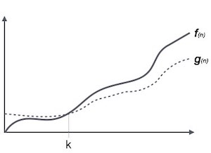
For example, for a function f(n)

Ω(f(n)) ≥ { g(n) : there exists c > 0 and n0 such that g(n) ≤ c.f(n) for all n > n0. }

Theta Notation, θ

The notation θ(n) is the formal way to express both the lower bound and the upper bound of an algorithm's running time. It is represented as follows −

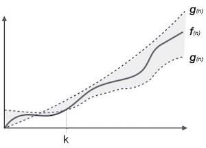
θ(f(n)) = { g(n) if and only if g(n) =  Ο(f(n)) and g(n) = Ω(f(n)) for all n > n0. }

Common Asymptotic Notations

Following is a list of some common asymptotic notations −

constant	−	Ο(1)
logarithmic	−	Ο(log n)
linear	−	Ο(n)
n log n	−	Ο(n log n)
quadratic	−	Ο(n2)
cubic	−	Ο(n3)
polynomial	−	nΟ(1)
exponential	−	2Ο(n)

Data Structures - Greedy Algorithms

An algorithm is designed to achieve optimum solution for a given problem. In greedy algorithm approach, decisions are made from the given solution domain. As being greedy, the closest solution that seems to provide an optimum solution is chosen.

Greedy algorithms try to find a localized optimum solution, which may eventually lead to globally optimized solutions. However, generally greedy algorithms do not provide globally optimized solutions.

Counting Coins

This problem is to count to a desired value by choosing the least possible coins and the greedy approach forces the algorithm to pick the largest possible coin. If we are provided coins of ₹ 1, 2, 5 and 10 and we are asked to count ₹ 18 then the greedy procedure will be −

• 1 − Select one ₹ 10 coin, the remaining count is 8

• 2 − Then select one ₹ 5 coin, the remaining count is 3

• 3 − Then select one ₹ 2 coin, the remaining count is 1

• 4 − And finally, the selection of one ₹ 1 coins solves the problem

Though, it seems to be working fine, for this count we need to pick only 4 coins. But if we slightly change the problem then the same approach may not be able to produce the same optimum result.

For the currency system, where we have coins of 1, 7, 10 value, counting coins for value 18 will be absolutely optimum but for count like 15, it may use more coins than necessary. For example, the greedy approach will use 10 + 1 + 1 + 1 + 1 + 1, total 6 coins. Whereas the same problem could be solved by using only 3 coins (7 + 7 + 1)

Hence, we may conclude that the greedy approach picks an immediate optimized solution and may fail where global optimization is a major concern.

Examples

Most networking algorithms use the greedy approach. Here is a list of few of them −

• Travelling Salesman Problem
• Prim's Minimal Spanning Tree Algorithm
• Kruskal's Minimal Spanning Tree Algorithm
• Dijkstra's Minimal Spanning Tree Algorithm
• Graph - Map Coloring
• Graph - Vertex Cover
• Knapsack Problem
• Job Scheduling Problem

There are lots of similar problems that uses the greedy approach to find an optimum solution.

Data Structures - Divide and Conquer

In divide and conquer approach, the problem in hand, is divided into smaller sub-problems and then each problem is solved independently. When we keep on dividing the subproblems into even smaller sub-problems, we may eventually reach a stage where no more division is possible. Those "atomic" smallest possible sub-problem (fractions) are solved. The solution of all sub-problems is finally merged in order to obtain the solution of an original problem.

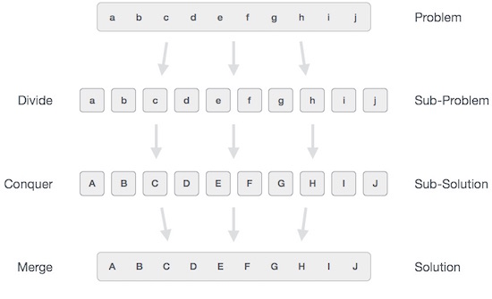
Broadly, we can understand divide-and-conquer approach in a three-step process.

Divide/Break

This step involves breaking the problem into smaller sub-problems. Sub-problems should represent a part of the original problem. This step generally takes a recursive approach to divide the problem until no sub-problem is further divisible. At this stage, sub-problems become atomic in nature but still represent some part of the actual problem.

Conquer/Solve

This step receives a lot of smaller sub-problems to be solved. Generally, at this level, the problems are considered 'solved' on their own.

Merge/Combine

When the smaller sub-problems are solved, this stage recursively combines them until they formulate a solution of the original problem. This algorithmic approach works recursively and conquer & merge steps works so close that they appear as one.

Examples

The following computer algorithms are based on divide-and-conquer programming approach −

• Merge Sort
• Quick Sort
• Binary Search
• Strassen's Matrix Multiplication
• Closest pair (points)

There are various ways available to solve any computer problem, but the mentioned are a good example of divide and conquer approach.

Data Structures - Dynamic Programming

Dynamic programming approach is similar to divide and conquer in breaking down the problem into smaller and yet smaller possible sub-problems. But unlike, divide and conquer, these sub-problems are not solved independently. Rather, results of these smaller sub-problems are remembered and used for similar or overlapping sub-problems.

Dynamic programming is used where we have problems, which can be divided into similar sub-problems, so that their results can be re-used. Mostly, these algorithms are used for optimization. Before solving the in-hand sub-problem, dynamic algorithm will try to examine the results of the previously solved sub-problems. The solutions of sub-problems are combined in order to achieve the best solution.

So we can say that −

• The problem should be able to be divided into smaller overlapping sub-problem.

• An optimum solution can be achieved by using an optimum solution of smaller sub-problems.

• Dynamic algorithms use Memorization.

Comparison

In contrast to greedy algorithms, where local optimization is addressed, dynamic algorithms are motivated for an overall optimization of the problem.

In contrast to divide and conquer algorithms, where solutions are combined to achieve an overall solution, dynamic algorithms use the output of a smaller sub-problem and then try to optimize a bigger sub-problem. Dynamic algorithms use Memorization to remember the output of already solved sub-problems.

Example

The following computer problems can be solved using dynamic programming approach −

• Fibonacci number series
• Knapsack problem
• Tower of Hanoi
• All pair shortest path by Floyd-Warshall
• Shortest path by Dijkstra
• Project scheduling

Dynamic programming can be used in both top-down and bottom-up manner. And of course, most of the times, referring to the previous solution output is cheaper than recomputing in terms of CPU cycles.

To be continued.........

In our next or upcoming blog we will starting from Basic of Data Structures and Algorithm.

so stay tuned and subscribe our youtube channel  Codin India